It would be really interesting to try to make a waveform that is fractal in nature, and actually sounds interesting and musical at whatever frequency you play it at. As you speed it up, some frequencies will go so high they become inaudible and new frequencies move into the audible range at the low end. In normal music, the pitches, effects, tempos and structures all happen at different timescales but in fractal music they would all interact with each other in interesting ways.
Archive for the ‘fractals’ Category
Fractal waveform
Tuesday, September 27th, 2011Interactive IFS
Monday, September 19th, 2011I want to write a program that allows you to explore Iterated Function System (IFS) fractals interactively by moving points around with the mouse.
There's a few different ways to do this, depending on what set of transformations you use.
IFS fractals usually use affine transformations, which encompass translations, rotations, dilations and shears. This can be done with 3 points per transformation - if one considers the points as complex numbers we have the transformation =ax + b\overline{x} + c")


i+c")
However, there are other possible transformations. We could reduce the number of control points to 2 and disallow non-orthogonal transformations, giving =ax + b")

We could move to quadratics  = ax^2 + bx + c")

 = ax^3 + bx^2+cx+d")
")
")
")
")
We can even go all the way to  = ax^2 + b\overline{x}^2 + c|x|^2 + dx + e\overline{x} + g")
I'd also like to be able to associate a colour with each transformation so that the colour of a point in the final image depends on the sequence of transformations that led to that point. Perhaps C_{transform}")

Fractals on the hyperbolic plane
Tuesday, August 30th, 2011Some amazing images have been made of fractal sets on the complex plane, but I don't think I've ever seen one which uses hyperbolic space in a clever way. I'm not counting hyperbolic tessellations here because the Euclidean analogue is not a fractal at all - it's just a repeated tiling.
The hyperbolic plane is particularly interesting because it is in some sense "bigger" than the Euclidean plane - you can tile the hyperbolic plane with regular heptagons for example. Now, you could just take a fractal defined in the complex plane and map it to the hyperbolic plane somehow, but that doesn't take advantage of any of the interesting structure that the hyperbolic plane has. It's also locally flat, so doesn't add anything new. If you use some orbit function that is more natural in the hyperbolic plane, I think something much more interesting could result. I may have to play about with this a bit.
Similarly, one could also do fractals on the surface of a sphere (a positively curved space - the hyperbolic plane is negatively curved and the Euclidean plane has zero curvature).
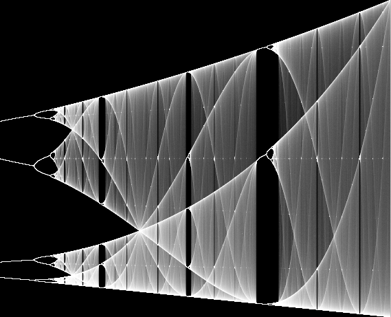
Bifurcation fractal
Thursday, August 18th, 2011I wrote a little program to plot the Bifurcation fractal when I was learning to write Windows programs from scratch - this is an updated version of it. Unlike most renderings of this fractal, it uses an exposure function to get smooth gradients and scatters the horizontal coordinate around the window so you get both progressively improvements in image quality and can see very fine details (such as the horizontal lines of miniature versions of the entire picture).
You can zoom in by dragging a rectangle over the image with the left mouse button, and zoom out by dragging a rectangle with the right mouse button.
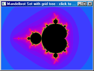
Arbitrary precision Mandelbrot sets
Tuesday, July 6th, 2010I added arbitrary precision arithmetic to my Mandelbrot zoomer. Surprisingly, the difficult part wasn't the arbitrary precision arithmetic itself, it was deciding when and how to switch from double-precision to arbitrary precision arithmetic. Because my program reuses data computed at one zoom level to speed up the computation of more deeply zoomed images, some images contained pixels computed using both methods. The trouble is, the two methods don't give the same results. In fact, after some experimentation I discovered that the problem was even worse than that: even using just the double-precision code, you get different results depending on the number of digits you use. So the point that was represented in my program by 0xffa615ce + 0x00000002i (using 10.22 bit fixed point) escaped after 548 iterations but the point 0xffa615ce00000000 + 0x0000000200000000i (using 10.54 bit fixed point) escaped after 384 iterations. The problem is that after every multiplication we shift the result right by the number of fractional bits, which performs a rounding operation. The images generated look reasonable but are actually only approximations to the true images that would be calculated if infinite precision were employed.
Having determined this, I realized it would be necessary to throw away all the points computed with lower precision once we started using a higher precision. This isn't as bad as it sounds, since (when zooming in by a factor of 2) the recycled points only account for 1/4 of the computed points but if we just threw them all out at once it would result in a visible artifact when passing through the precision boundary - the entire window would go black and we'd restart calculation from scratch. I wanted to avoid this if possible, so I started thinking about convoluted schemes involving restarting a point if its 3 sibling points were of higher precision. Then I realized that I could just recycle the points but keep their colours when splitting blocks to a new precision boundary, avoiding the glitch. There are still some artifacts while the image is being computed, but they are less jarring.
Finally there was the problem of interfacing with double-precision floating-point numbers. The Mandelbrot set is contained entirely within the circle |c|<2 and in this range a double has 52 bits of fractional precision. But if we replace the 10.22 and 10.54 bit fixed point numbers with doubles, we'll have a region of blockiness where we need 53 or 54 bits but only have 52. Rather than having two sorts of 64-bit precision numbers, I decided to simplify things and have 12 integer bits in my fixed point numbers. The program is very slow when it switches into arbitrary precision mode - it's barely optimized at all. The 96-bit precision code is currently has a theoretical maximum speed of about 92 times slower than the SSE double-precision code (190 million iterations per second vs 2 million). It could be significantly faster with some hand assembler tuning, though - I have a 96-bit squaring routine that should speed it up by an order of magnitude or so. All of the multiplications in the Mandelbrot inner loop can be replaced with squarings, since [latex]2xy = (x+y)^2 - x^2 - y^2[/latex]. Squaring is a bit faster than multiplication for arbitrary precision integers, since you only need to do [latex]\displaystyle \frac{n(n+1)}{2}[/latex] digit multiplications instead of [latex]n^2[/latex]. Given that we are calculating [latex]x^2[/latex] and [latex]y^2[/latex] anyway and the subtractions are very fast, this should be a win overall.
Improved GPU usage for fractal plotter
Sunday, November 1st, 2009I've been tinkering with my fractal plotter again. One thing that annoyed me about it was the pauses when you zoomed in or out past a power of 2. I thought this was due to matrix operations until I did some profiling and discovered that it was actually dilation (both doubling and halving) of the "tiles" of graphical data to which squares are plotted and which themselves are painted to the screen.
This is work that can quite easily be done on the GPU, without even having to resort to pixel shaders, by using the ability to render to a texture. Here is the result and here is the source. In order to do this I moved all the tiles to video memory (default pool instead of managed pool) and used ColorFill() to actually plot blocks instead of locking and writing directly to textures. All this adds up to much more CPU time available for fractal iterations.
Another change is that instead of an array of grids of tiles, I've switched to using a grid of "towers" each of which is itself a tile and can point to 4 other towers. This simplifies the code somewhat.
There is still some glitchiness when zooming but it is much less noticable now.
This reminds me of something I meant to write about here. When I originally converted my fractal program to use Direct3D, I figured that locking and unlocking textures was probably an expensive operation so rather than locking and unlocking every time I needed to plot a square, I kept them all locked most of the time and just unlocked them to paint. However, it turns out that this "optimization" was actually a terrible pessimization - now all the tiles were dirtied each frame and had to be copied from system memory to video memory for each paint, and because of the locking nothing else could happen during that time. I was able to get a big speed up by locking and unlocking around each plot operation - that caused only the parts of tiles that were actually plotted on to be dirtied. It just goes to show that when optimizing you do have to be careful to actually measure performance and see where the slow bits really are.
Rotating fractal
Thursday, October 29th, 2009Last year, I wrote about a way to make rotating fractals. I implemented this and here is the result:
The equation used was z <- z1.8 + c, and the branch cut varies from 0 to ~10π.
A trip around the cardioid
Tuesday, October 27th, 2009Take a point that moves around the edge of the main cardioid of the Mandelbrot set, and plot orbits with values of c close to that point. You end up with this:
It can be thought of as a sequence of cross-sections of the Buddhabrot.
Memory handling for fractal program
Sunday, August 9th, 2009I have been poking again at my fractal plotting program recently. The latest version is available here (source). I've added multi-threading (so all available cores will be used for calculation) and Direct3D rendering (which makes zooming much smoother and allows us to rotate in real time as well with the Z and X keys - something I've not seen any other fractal program do). There is still some jerkiness when zooming in or out (especially past a power-of-two boundary) but it's greatly reduced (especially when there's lots of detail) and with a little more work (breaking up the global matrix operations) it should be possible to eliminate it altogether.
The linked grid data structure in the last version I posted worked reasonably well, but it used too much memory. At double-precision, every block needed 72 bytes even after it had been completed. This means that an image that covered a 1600x1200 screen with detail at 16 texels per pixel for anti-aliasing would use more than 2Gb. I could use a different block type for completed points but there would still need to be at least 4 pointers (one for each direction) at each point, which could take 500Mb by themselves.
So I decided to switch to a data structure based on a quadtree, but with some extra optimizations - at each node, one can have not just 2x2 children but 2n by 2n for any positive integer n. When a node contains 4 similar subtrees (each having the same size and subnode type) it is consolidated into a 2n+1 by 2n+1 grid. If we need to change the type of one of the subnodes of this grid, we do the reverse operation (a split). In this way, if we have a large area of completed detail it will use only 4 bytes per point (storing the final number of iterations). This works much better - memory usage can still be quite high during processing (but seems to top out at ~700Mb rather than ~2Gb for the linked grid data structure) and goes right back down to ~200Mb when the image is completed (only about 35Mb of which is the data matrix, the rest is Direct3D textures).
One disadvantage of the grid tree method is that it doesn't naturally enforce the rule preventing 4 or more blocks being along one side of one other block. That rule is important for ensuring that we don't lose details that protrude through a block edge. However, this turns out to be pretty easy to explicitly add back in. This gives a more efficient solid-guessing method than I've seen in any other fractal program (by which I mean it calculates the fewest possible points in areas of solid colour).
This data structure was surprisingly difficult to get right. The reason for this is that with all the splitting and consolidating of grids, one must avoid keeping grid pointers around (since they can get invalidated when a split or consolidation happens in a nearby part of the tree). That means that many algorithms that would be natural to write recursively need to be written iteratively instead (since the recursive algorithm would keep grid pointers on the call stack).
Another tricky thing to get right was the memory allocation. My first attempt just used malloc() and free() to allocate and deallocate memory for the grids. However, the way grids are used is that we allocate a whole bunch of them and then deallocate most of them. However, they are quite small and the ones that don't get deallocated are spread throughout memory. This means that very little memory can be reclaimed by the operating system, since nearly every memory page has at least one remaining block (or part of one) on it.
The problem here is that the malloc()/free() interface assumes that a block, once allocated, never moves. However, grids turn out to be quite easy to move compared to general data structures. This is because the grid tree is only modified by one thread at once (it must be, since modifying it can invalidate any part of it) and also because we know where all the grid pointers are (we have to for split and consolidate operations). Only a dozen or so different grid sizes are currently used in practice, so it's quite practical to have a separate heap for each possible grid size. If all the objects in a heap are the same size, there's an extremely simple compaction algorithm - whenever we delete an item, just move the highest item in the heap down into the newly free space. So a heap consists of a singly-linked list of items. These are allocated in chunks of about 1Mb. Each chunk is contiguous region of memory, but chunks within a heap don't have to be contiguous. This allows the heaps to interleave and make the best use of scarce (on 32-bit machines) address space.
Sounds simple enough but again there turned out to be complications. Now it's not just split and consolidate that can invalidate grid pointers - now deleting a grid can also invalidate grid pointers. This means more recursive algorithms that need to be made iterative (such as deleting an entire subtree) and certain operations need to be done in a very specific order to avoid keeping more grid pointers around than are necessary. I now understand why such techniques are so rarely used - they're really difficult to get right. I do think that a general garbage-collected heap would be slower and use more memory than this special purpose allocator, but I'm not sure if difference would be large enough to make all this effort worth it. Perhaps someone will port my code to a garbage-collected language so the performance can be compared.
Sound for fractal program
Saturday, August 8th, 2009I'd like to be able to add some kind of sound output to my fractal program. What I'd like to do is generate a click every time a point is completed. So, when it's working on a difficult area it would emit a clicking sound but when it's finishing a lot of points it would generate white noise. The principle is very similar to that of a geiger counter's audio output.
This is trivial to do under DOS, but in Windows it is surprisingly difficult. Ideally we want to generate a waveform at 44.1KHz. When we finish a point, we flip the current sample in the audio buffer between its maximum and minimum positions. The problem is determining what the current sample should be (or, alternatively, moving a pointer to the next sample 44,100 times per second). What we need is a high-resolution timer, but none of the high-resolution timers seem to be particularly reliable. timeGetTime() is too low-resolution. QueryPerformanceCounter() has bugs on some systems which cause it to skip backwards and forwards a few seconds on occasion. The RDTSC CPU instruction isn't guaranteed to be synchronized between CPUs, and its count rate may vary due to power saving features on some CPUs. Another possibility is reading the playback cursor position from DirectSound, but that is unreliable on OSes before Vista.
What I may end up doing is faking it - measure the average number of blocks completed over some small period of time and use that to generate the clicks via a Poisson distribution.