Reenigne blog

Lots of videos have been made of zooms into the Mandelbrot set. These videos almost all follow the same pattern. The initial image is the familiar one of the entire set. One zooms in on some tendril or other, gathering details, passing various minibrots and possibly some embedded Julia sets on the way until one reaches a final minibrot and the zoom stops.

The reason for this is that these sequences are relatively quick to calculate, they show a variety of the different types of behaviors that the Mandelbrot set has to offer, and they have a natural endpoint which causes the video not to seem like it has been cut off part-way through.

If we relax these conditions, what interesting zoom sequences open up to us?

To answer this question requires classification of the complex numbers according to the roles they play in the Mandelbrot set.

The first taxon separates exterior points (whose z sequences are unbounded, example: +1), interior points (limit of z sequence is a finite attracting cycle, example: 0) and boundary points (all other z sequence behaviours). Zooming into either of the first two will leave us with an image of uniform colour after a finite amount of time. Most zoom movies actually target the second of these.

Zooming in on the boundary will leave us with an infinite sequence of "interesting" images, so let's explore this group further. The second taxon separates shore points (those which are on the edge of an atom), Feignbaum points (which are at the limit of a sequence of atoms of increasing period) and filament points (all other boundary points).

Feignbaum points make quite interesting infinite zoom sequences. The canonical example is ~-1.401155, the westernmost point of the main molecule. Each time you zoom in by a factor of ~4.669201, the lakes look the same but the the filaments get denser. Filaments connect to molecules at these points. These are the only places filaments attach to the continent but each mu-molecule has one additional filament emerging from its cardioid cusp.

Filament points can be divided into two types based on orbit dynamics - those whose orbit is chaotic (irrational external angle) and those whose orbit converges to a finite repelling cycle. The latter includes two subtypes - branch points (where there are more than one but fewer than infinity paths to other points in the set) and terminal points (where there is only one). Well-known terminal points include -2 and +i. Zooming into terminal points and branch points gives a video which is infinite but which devolves into very same-y spirals after a short time as the mu-molecules shrink to less than a pixel.

I don't know an exact formula for any chaotic filament points, but they're easy to find using a fractal plotter - just zoom in, keeping away from any mu-molecules, branch points and terminal points. As with terminal and branch points, the minibrots tend to shrink to less than a pixel quite quickly, so the images obtained will become same-y after a while - the structures formed by the filaments tend to look like L-system fractals.

Shore points can be divided into two categories, parabolic points and Siegel points. Parabolic points come in two flavors, cardioid cusps (the point of maximum curvature of a cardioid, example: +0.25) and bond points (where two atoms meet, example: -0.75). If you zoom in a cusp you'll technically always have detail on the screen but the picture gets very boring very quickly as the cusps shrink to sub-pixel widths.

This leaves the Siegel points. You can find these by zooming into the edge of an atom but avoiding the cusps. For example:

1. Start off with the large circle to the west (call it A) and the slightly smaller circle to the north (call it B).
2. Zoom in until you can pick out the largest circle C between A and B on the boundary of the set.
3. Rename B as A and C as B.
4. Go to step 2.

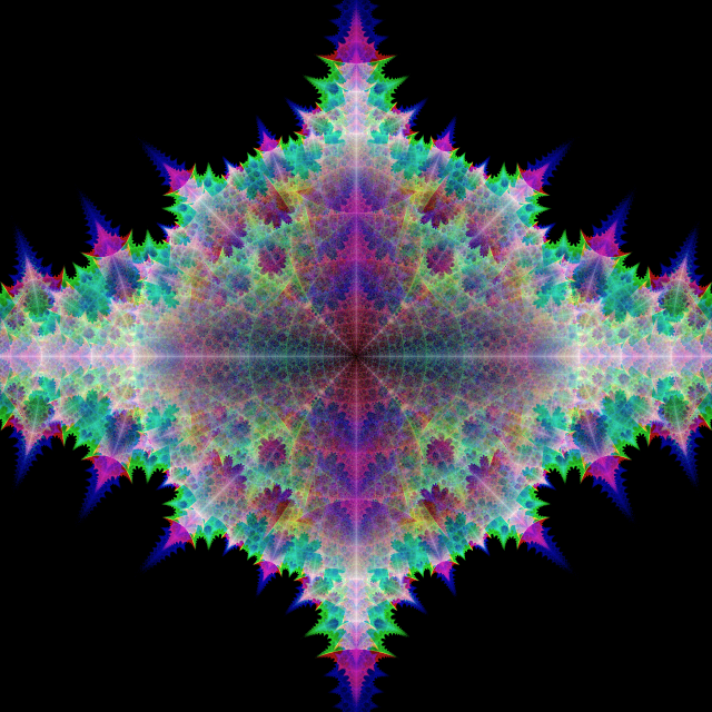
This particular algorithm takes you to the point whose Julia set is known as the Siegel disk fractal, which is about -.390541+.586788i.

All points on the boundary of the continent cardioid can be found using the formula . For rational , this gives a parabolic point and for irrational this gives a Siegel point (a point whose Julia set has Siegel discs). The "most irrational" number (in the sense that it is least well approximated by rational numbers) is the Golden ratio . The Siegel point corresponding to this number is the point reached by the algorithm given above. In some sense then, this area is the most difficult area of the Mandelbrot set to plot, and indeed if you attempt to zoom into it you'll quickly discover that you have to increase the maximum number of iterations exponentially to avoid losing detail. I don't think it's really practical to explore this area very far without a Mandelbrot set program that can do SOI, such as Fractint, Fractal Witchcraft (which is a pain to get working now as it's a DOS program), almondbread (which is a pain to get working now as one of its prerequisites seems to no longer be available) or the program I'm writing.

If you could zoom a long way into it, what would the Siegel area of the Mandelbrot set look like? Well, we know the part inside the cardioid is inside the set. We also know it's not a bond point so at least part of the remainder is outside the set. The pattern of circles on the cardioid is self-similar (it's related to Farey addition) so the continent part would look similar to a shallow zoom on the same point. The rest is a bit hazy, though. My experiments suggest that the density and relative size of mu-molecules gets greater as one zooms in on this area, so an interesting question to ask is what the limit of this process is? Would the area outside the continent be covered with (possibly highly deformed) tesselating mu-molecules, leading to a black screen? Or would only part of the image be covered by mu-molecules, the rest being extremely dense filament structures? Both possibilities seem to be compatible with the local Hausdorff dimension being 2. Either way I suspect there are some seriously beautiful images hiding here if we can zoom in far enough.

Summary of the taxonomy:

• Exterior points (example: infinity)
• Member points
  • Interior points
    • Superstable points (examples: 0, -1)
    • Non-superstable points
  • Boundary points
    • Filaments
      • Repelling points
        • Terminal points (examples: -2, +/- i)
        • Branch points
      • Chaotic, irrational external angle filaments
    • Feignbaum points (example: ~-1.401155)
    • Shore points
      • Parabolic points
        • Cardioid cusps (examples, 0.25, -1.75)
        • Bond points (examples, -0.75, -1 +/- 0.25i, -1.25, 0.25 +/- 0.5i)
      • Siegel points (example: ~= -.39054087021840008+.58678790734696872i)

I'm writing a super-fast, super-accurate Mandelbrot set plotter. This one is unusual in that no explicit iteration limit is ever set - it will keep iterating any point until it either escapes or is determined to be in the set. This works pretty well and produces much sharper cusps than any other program I've seen.

However, the downside is that it can take an arbitrarily long to determine if any given point is in the set or not. Points on the edge of the set are (as always) the particularly tricky ones - some of them exhibit chaotic behavior for a very long time before becoming periodic or escaping.

Currently I use two methods for determining if a point is in the set. I have explicit formulae for the main cardioid and the period-2 bulb, and I look for periodic orbits using Floyd's algorithm.

I'm wondering if a third method might be practical - one that determines if a point is in the set without waiting for it to become periodic. Here's the method I'm considering.

Let the Mandelbrot iteration function f(z) = z² + c. Suppose we have a point c, and we suspect that it might be periodic with period N. We can determine if it is or not by finding a point z_f that is unchanged under N applications of f, i.e. a solution to f^N(z_f) = z_f. There will generally be 2^N such solutions, of which only N will be relevant to the case at hand. However, if we have a z that is likely to be near one of these fixed points we should be able to converge on one of them quickly by using Newton's method or something similar.

Once we have our fixed point, we take the derivative of f^N with respect to c and evaluate it at z_f. This is easy to do numerically - just evaluate f^N at z_f and a nearby point, take the difference and divide by the original distance. If the modulus of the result is 1 or less, then the attractor is stable and c is in the set. If it isn't, the point could still be in the set as we might have picked the wrong z_f or N - that is we are likely to get false negatives but no false positives using this method (which is exactly what we want - if we get a false negative we can
iterate some more, try a new N and/or a new z_f and eventually get the right answer).

Working through these steps symbolically gives us closed form solutions for the period-1 and period-2 attractors but if we try it for period 3 we get a polynomial of order 6 in z (2³ = 8 minus the two from factoring out the period-1 attractor) - I'm not sure if we can get a closed form solution for period-3 attractors from this.

The tricky part is choosing an appropriate N and an approximation to z_f for any given point. I think the way to do it is this: whenever we find a periodic point with Floyd's algorithm, iterate a further N times to figure out the period, and store the period and fixed point. When we start a new set of iterations on a point, check to see if any neighbouring points are periodic. If they are, try this method using the N from that point and the z_f (appropriately adjusted for the new c). When we find a periodic point this way, we store the found N and z_f just as for Floyd's algorithm.

A good way to speed up a Mandelbrot set plotter is to eliminate the main cardioid and the largest circle. It turns out that there are simple equations for these, which can be found if you know that the cardioid consists of all the points which converge to a single point and the largest circle consists of all the points which converge to a cycle of period 2.

First the main cardioid. For each c, we can find the fixed point of iteration such that . There are two solutions, . Then we can look at what happens when we iterate a nearby point . If then the fixed point is stable. It turns out that this only happens for the solution, so points in the cardioid are , with equality for the boundary.

Having to compute a complex square root is a bit ugly, though - can we do better? It turns out that we can. It's a fiddly calculation but if you multiply out all the square roots and simplify, you can get the formula .

For the period-2 circle, we solve and eliminate the period-1 solutions to get . In this case, both solutions are equally valid, since the cycle consists of both. Picking one and doing the same derivative analysis (this time applying two iterations) gives us the circle with center at -1 and radius 1/4.

The video I made for Saturday's post made me wonder what the picture would look like if you didn't have a branch cut at all - if you make the logarithm function generate all of its multiple values (or equivalently, choose a sheet of the Riemann surface at random). Computers can't count up to infinity so the random method must be used. We can't make all the sheets equally likely as their number is unbounded so we need to pick some distribution. I chose a method that's rather simple to implement - I just roll a (virtual) dice until a 1 or a 6 comes up, and subtract the number of 2s and 3s from the number of 4s and 5s (a 1D random walk). That makes positive and negative numbers equally likely, but makes small (positive or negative) numbers more likely than large ones.

Here is the result:

The infinite tower is transformed into a fractal fern-like structure. I was surprised at how different this looked from the second image on this post - while the non-principal branches are not visited very often, they cover a lot of space so make a lot of difference to the image.

The second image in this post was quite popular, so I decided to make a movie out of it.

There aren't really many parameters in the equations used to make this image, though - (the functions are just negative, exponential and logarithm). The colouring is arbitrary but modifying it wouldn't make a very interesting movie. The zoom factor is fairly arbitrary as well but zooming very much in or out would make the image take much longer to render (besides which, zooming movies have been done to death). About the only other arbitrary thing about the image is the choice of branch cut for the logarithm.

This describes a way of adjusting the branch cut in a continuous way, and this is the movie I made by adjusting theta from -4.5 to +4.5 radians:

High quality 640x480 11Mb DivX avi version.

This took about three days to render. I could have done it faster, but my laptop gets uncomfortably warm when both its cores are fully utilized. Also, a problem with Vista networking was causing the other machine I was using to keep getting disconnected from my laptop every few frames.

A commenter wondered what the images on Saturday's post would look like using a sixth root of unity instead of a fourth. I am happy to oblige. With ω=e^πi/3, this is the image with the operations z+ω, ωz, ω^z:

And this is the image with the operations z+ω, ωz, z^ω:

More variations:

Red: z->z+i
Green: z->iz
Blue: z->i^z:

Same, but with blue: z->zⁱ:

A movie can be thought of as a three-dimensional array of pixels - horizontal, vertical and time. If you have such a three-dimensional array of pixels, there are three different ways of turning it into a movie - three different dimensions that you can pick as "time". For movies of real things this probably isn't a very interesting thing to do, but for movies of mathematical objects like the one I made yesterday, there may be mathematical insights to be gained from "reslicing" a movie.

So, here is yesterday's movie with the x and time coordinates swapped:

Higher resolution version (8Mb 640x480 DivX).

And here it is with the y and time coordinates swapped (and also rotated to landscape format):

Higher resolution version (8Mb 640x480 DivX).

Higher quality 10Mb 640x480 DivX version here.

This is a generalization of the second picture from yesterday's post, varying the coefficient of i from e^-4.5 to e^4.5. It also demonstrates how this picture is related to the third picture from Monday's post.

1.35 trillion points were calculated to make this movie, taking 4 CPUs with 6 cores most of a day (it was going to take nearly 4 days, but I decided to use most of the other computers in the house as a render farm).

Generated by a program similar to the last two pictures on Monday's post, but the functions are , and . Don't plot a point if the last operation was , and colour points according to the operation used 5 iterations ago.

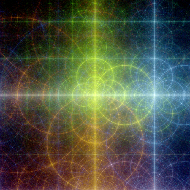
Similar to the third image on Monday's post, but when we multiply by we also multiply by the golden ratio = 1.618... Most the rectangles you see in this image are golden rectangles, which are supposedly the most aesthetically pleasing.